Making a photorealistic image in code
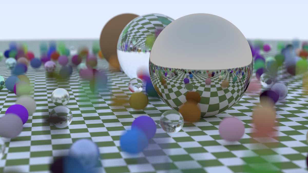
Programming a computer to make a photorealistic image is a very cool party trick. Thinking about the problem from first principles, it’s not clear what you need to get this thing working. I mean, there’s a clue in the name - it’s tracing rays. The gives us a clear indication that we will be following light rays along in a 3d scene, sure. But what was not clear to me is how much is needed, how much detail, when modelling the light-matter interaction to get a result that looks good. It turns out that the answer is: surprisingly little. Here’s what I made by following an amazing free three-book series by Peter Shirley, Trevor David Black and Steve Hollasch: Ray Tracing in One Weekend.
Not only is ray tracing a fun project because the end results are beautiful, even at minimal effort. It’s a great project because it lends itself perfectly to the reward loop where you write-compile-view-iterate. It’s perfect for nice little seratonin boosts, and because the render time can be non-negligible you even get a bit of down time in betweem renders if you want it.
The Ray tracing in one weekend series
Ray tracing in one weekend (RTOW from here on) does an amazing job of showing you exactly how to implement a ray tracer in C++. You don’t even need to know C++ to any serious level if you want to follow it. The phylosophy is consistently such that it’s the bare minimum needed, but not less than that. It’s very hard to pull something like that off and the series is amazing for doing it perfectly. And it’s free!
At work, I’ve been using ray tracers in various forms for a while now. There are a bunch of famous serious implementations like pbrt or Pixar’s RenderMan and when working with Blender (which I’ve loved since my PhD days) there’s Cycles but I never put any serious thought into how this thing works. Having gone thorough a basic example, I have a much better understanding into some of the knobs I mindlessly twisted in Blender to change the visual quality of outcome.
In RTOW you build the ray-tracer math from the ground up. In the book you implelment the entire stack needed to describe vector math and some linear algebra operations (because of course it’s linear algebra. EVERYTHING is.). I opted to implement things in Rust. Both because it made it a bit more of a challenge (compared to copying the code snippets) and because I wanted to see if I could port things over to WASM once again. I did.
How does basic ray tracing work?
The fundamental problem of 3D graphics is projecting a three-dimensional world onto a two-dimensional grid of pixels. In “rasterization” (the technique used by almost all real-time video games), we take triangles and project them onto the screen. It’s incredibly fast, but it struggles with things that light does naturally: soft shadows, reflections, and complex refraction.
Ray tracing flips the script. Instead of projecting triangles to the screen, we shoot “rays” from the eye (or camera) through each pixel and into the scene. We ask: “What does this ray hit?”
The Geometry of a Ray
A ray is essentially a mathematical function of a 1D parameter $t$. If we have an origin point $\vec{A}$ and a direction vector $\vec{b}$, any point $\vec{P}$ along that ray can be described as:
$$ \vec{P}(t) = \vec{A} + t\vec{b} $$As we vary $t$, the point $\vec{P}(t)$ moves along the line. If $t > 0$, the point is in front of the camera; if $t < 0$, it’s behind us. Our task is to find the smallest positive $t$ where this ray intersects an object in our scene.
Anything you want to render, as long as it’s a sphere
So we need to solve for t, so we need a concrete geometry. We start with only spheres. To render a sphere, we simply need to find the intersection of this ray and the equation for a sphere. If a sphere has center $\vec{C}$ and radius $r$, then any point $\vec{P}$ on the surface of the sphere satisfies the following equation:
$$ (\vec{P} - \vec{C}) \cdot (\vec{P} - \vec{C}) = r^2 $$This says that the square of the distance from the center to any point on the surface is equal to the radius squared. By substituting our ray equation $\vec{P}(t) = \vec{A} + t\vec{b}$ into the sphere equation, we get a quadratic equation in terms of $t$:
$$ (\vec{A} + t\vec{b} - \vec{C}) \cdot (\vec{A} + t\vec{b} - \vec{C}) = r^2 $$Expanding this out, we get:
$$ t^2(\vec{b} \cdot \vec{b}) + 2t(\vec{b} \cdot (\vec{A} - \vec{C})) + (\vec{A} - \vec{C}) \cdot (\vec{A} - \vec{C}) - r^2 = 0 $$So we need to solve a quadratic. If the discriminant ($b^2 - 4ac$) is positive, the ray hits the sphere in two places (entering and exiting). If it’s zero, it grazes the edge. If it’s negative, we missed entirely. We pick the smallest positive $t$, calculate the surface normal at that point (the vector pointing straight out from the center), and use it to determine the color.
Scattering and reflections
What makes ray tracing “photorealistic” is how it handles materials. When a ray hits a surface, it doesn’t just stop and return a color. It asks the surface: “How do you reflect light?”
This leads to a recursive process. The color of a pixel is not a static value; it is the sum of the light gathered by a ray as it bounces around the scene.
1. Diffuse (Lambertian) Surfaces
Matte surfaces, like a brick or a piece of paper, scatter light in random directions. In our code, when a ray hits a diffuse surface, we generate a new ray starting at the hit point and pointing in a random direction within a hemisphere aligned with the surface normal. We then recursively call our color function for this new ray and scale the result by the material’s albedo (its reflectivity).
2. Metallic Surfaces
Metal is different. A perfect mirror reflects light such that the angle of incidence equals the angle of reflection. We can calculate this reflected vector $\vec{r}$ using the incident vector $\vec{v}$ and the surface normal $\vec{n}$:
$$ \vec{r} = \vec{v} - 2(\vec{v} \cdot \vec{n})\vec{n} $$In practice, few metals are perfect mirrors. We can simulate “fuzzy” reflections by adding a bit of randomness to the endpoint of the reflected vector, controlled by a “fuzziness” parameter.
3. Dielectrics (Glass and Water)
Glass reflects and refracts. Some of the ray reflects, and some of it refracts at an angle given by Snell’s Law:
$$ \eta \cdot \sin(\theta) = \eta' \cdot \sin(\theta') $$Where $\eta$ and $\eta’$ are the refractive indices of the two media. Implementing this in code requires handling the case of “Total Internal Reflection”—where the light is hitting the boundary at such a shallow angle that it cannot exit and must reflect. We also use “Schlick’s Approximation” to simulate how glass becomes more reflective when viewed at a grazing angle.
Detailed Transactions: The Life of a Ray
To better understand how a single pixel’s color is calculated, let’s look at the “transaction log” of a single ray as it bounces through the scene. Each bounce is a transaction between the ray and a material, modifying its energy until it either finds a light source or is killed by a recursion-limiting parameter.
| Bounce # | Material Hit | Action Taken | Color Attenuation | Remaining Energy |
|---|---|---|---|---|
| 1 | Glass Sphere | Refract | (1.0, 1.0, 1.0) | 100% |
| 2 | Metal Sphere | Reflect | (0.8, 0.6, 0.2) | 80% |
| 3 | Matte Ground | Scatter | (0.5, 0.5, 0.5) | 40% |
| 4 | Background Sky | Terminate | (0.5, 0.7, 1.0) | 20% (Final) |
Implementation in Rust
I chose Rust for this project for the same reasons I chose it for the Barnes-Hut simulation. It offers the performance of C++ but with some modern tooling and safety. And also (most importantly) because of fashion…
In a ray tracer, you are doing a lot of linear algebra. You need a fast Vec3 implementation. In Rust, we can use operator overloading to make our math look like math.
impl Add for Vec3 {
    type Output = Vec3;

    fn add(self, other: Vec3) -> Vec3 {
        Vec3 {
            x: self.x + other.x,
            y: self.y + other.y,
            z: self.z + other.z,
        }
    }
}

impl Vec3 {
    pub fn dot(self, other: Vec3) -> f64 {
        self.x * other.x + self.y * other.y + self.z * other.z
    }
}
Fearless Parallelism
Ray tracing is what computer scientists call “embarrassingly parallel”. Every pixel on the screen is independent of every other pixel. To calculate the color of pixel (10, 10), I don’t need to know anything about pixel (10, 11). Nevertheless this isn’t tackled in the original book implementation and I wanted to try and add it.
In many languages, adding multi-threading to a project involves a week of debugging race conditions and deadlocks. In Rust, I used the Rayon crate. But for Rayon to work, the objects in our scene must be thread-safe. This is where Rust’s Sync and Send traits come into play.
Sendguarantees that we can move our data between threads.Syncguarantees that multiple threads can safely share references to the same data.
By marking my Hittable trait (the interface for anything a ray can strike) as Sync, I can share the entire world across all my CPU cores. The compiler ensures that our scene is read-only during the render, making the parallelization as simple as changing a standard iterator into a .into_par_iter().
Below is the main render loop using this paralled iteration technique.
// Parallelizing the render loop with Rayon
(0..image_height).into_par_iter().rev().for_each(|j| {
    let mut line_buffer = Vec::new();
    for i in 0..image_width {
        let mut pixel_color = Color::new(0.0, 0.0, 0.0);
        for _ in 0..samples_per_pixel {
            let u = (i as f64 + random_double()) / (image_width - 1) as f64;
            let v = (j as f64 + random_double()) / (image_height - 1) as f64;
            let r = camera.get_ray(u, v);
            pixel_color += ray_color(&r, &world, max_depth);
        }
        line_buffer.push(pixel_color);
    }
    // Write line_buffer to file...
});
Going from one core to sixteen cores on my machine reduced the render time from several minutes to just a few seconds.
WASM: Bringing the Rays to the Browser
One of the most compelling reasons to use Rust for a project like this is its first-class support for WebAssembly (WASM). In my Barnes-Hut post, I included a live demo running directly in the browser.
For the browser-side implementation, I used the Leptos framework. Leptos is a web framework for building reactive UIs (a Rust React). Using its component-based architecture, I was able to build the “Render” button and the canvas integration that displays the ray-traced result in real-time.
However, moving from a desktop CLI tool to a browser-based renderer introduced a significant hurdle: parallelism.
On the desktop, as we saw, Rayon makes multi-threading trivial. But the browser’s execution model is fundamentally different. While Web Workers exist, they don’t share memory in the same way that threads do on a native OS. In a standard WASM build, you are effectively locked into a single-threaded world.
The Parallelism Paradox in the Browser
In native Rust, Rayon uses a work-stealing scheduler to distribute tasks across all available CPU cores. In WASM, Rayon doesn’t work out of the box because the underlying primitives—threads and atomic memory operations—require a specific environment.
To get true parallel rendering in the browser, you have to navigate a maze of security requirements. You need to enable SharedArrayBuffer support, which requires setting specific “Cross-Origin” headers on your web server. Even then, you need a specialized toolchain like wasm-bindgen-rayon to bridge the gap between Rust’s threads and JavaScript’s workers.
For this initial foray into the browser, I opted for a single-threaded render. An image that takes 5 seconds on my desktop takes nearly a minute in the browser. Having many cores is great, and it’s much better when we can actually use them.
Results
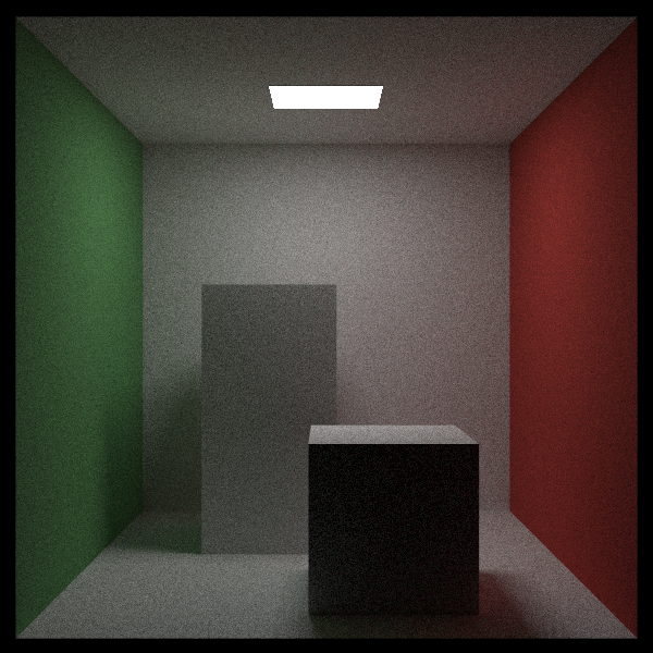
The final result of the first book is the one I included on the top of this post. Going into the second book adds a second shape: a rectangle (which we turn to a box). This allows us to model a famous graphics benchmarking scence called the Cornell Box. We also add a direct light source to this scene as you can see below.
There are many subtle features to the render I didn’t describe in detail. In the first image we can see things like Texture Mapping which allow us to map a 2D image onto a 3D sphere, Motion Blur in which there is motion in the sphere that shows up as a smeared object, Depth of focus which is dictated by the size of the lens aperture. There are also some techniques to speed up renders by limiting the search space where we try to find an object that is hit by a ray. Here we implemented BVH (Bounding Volume Hierarchies) which is a spatial data structure (much like the QuadTree in my Barnes-Hut post) that allows us to skip large groups of objects, bringing the cost down to $O(\log n)$.
There’s a lot more to explore in this world and I absolutly loved this project. Highly recommended. Check out the code, and the original book from which I took the implementation.